
If we want to understand economic fluctuations and business cycles, we need a disciplined way of thinking about how the nominal economy (denominated in current-valued dollars, e.g. market prices and interest rates) interacts with the real economy (denominated in dollarless quantities, e.g. unemployment and output). Economists have a pretty good model for this: the aggregate demand and aggregate supply (AD-AS) model.
No model is perfect, but in terms of parsimony and explanatory power, the AD-AS model is a very useful tool. It’s particularly helpful for understanding the economic forces that determine inflation and economic growth. Since economic growth makes people better off and inflation doesn’t, untangling these effects is important.
Aggregate demand describes the nominal (money-using) economy. It starts with the equation of exchange expressed in growth rates: the growth rate of effective monetary expenditures (gM+gV) equals the growth rate in nominal income (gP+gY). Aggregate demand shows all combinations of inflation (gP) and real output growth (gY) consistent with a given rate of nominal spending growth (gM+gV). If nominal spending is growing at, say, 5 percent, it must be the case that the sum of inflation and real output growth totals 5 percent.
By itself, this doesn’t tell us what inflation and economic growth will be. We need to incorporate the supply side. There are two relevant time horizons for modeling aggregate supply: the long run and the short run.
In the long run, all prices in the economy can adjust to clear markets, meaning the economy is producing at its maximum sustainable potential. Output growth each year is determined by non-monetary factors: increases in the labor supply, greater capital availability, new ideas and technology, and improvements in regulations and institutions. In the United States, historical real output growth usually fell between 2 and 3 percent.
In the short run, producers might expand output in response to higher prices. But those producers also know that there are two possible causes for higher prices: more real demand for their product or unanticipated money growth. If a car dealership experiences greater-than- anticipated sales growth for two straight months, does that mean car buyers are willing to offer more real resources than before? Or is it a funny-money effect, driven by central bank policy? Only the former scenario justifies increased production. If it’s the latter, rather than ordering more cars from the factory to increase sales to the public, the car dealership should just raise prices. Economists call this the signal-extraction problem: it’s costly to discover from rising prices (the signal) whether the underlying cause is real or nominal (the noise). Sometimes, unexpectedly loose money can trick producers into supplying more output than justified by the real economic fundamentals.
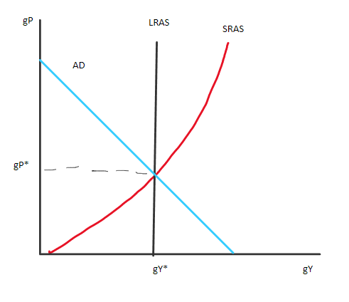
We can express all this graphically. Below is the canonical AD-AS model. Inflation is on the y-axis. Real output growth is on the x-axis. Aggregate demand is a line with a slope of -1: all combinations of inflation and real output growth that map on to a constant level of nominal income growth. Long-run aggregate supply is a vertical line: economic fundamentals don’t depend on monetary factors, and hence inflation. Short-run aggregate supply captures the signal extraction problem. It is an upward-sloping curve that gets increasingly steep as inflation rises since producers eventually run into real resource constraints. Machines can only run so fast and laborers work so hard. Especially when we’re beyond our long-run sustainable growth rate, producing faster gets increasingly hard.
Aggregate Demand and Aggregate Supply
Here’s the takeaway: In the short- to medium-run, aggregate demand expansion can temporarily cause economic booms. If the central bank surprises markets with excess liquidity, we can be fooled into producing more. In the long run, however, we get wise to the game. Once everyone learns about the ongoing easy monetary policy (higher money growth), output growth slows down and inflation rises. The only permanent effect of running the printing presses is higher inflation. Creating money isn’t the same thing as creating wealth.
Poor aggregate demand management by policymakers may result in economic turmoil. For example, a big spike to money demand (and hence a fall in gV) can throw a wrench in the economy’s gears. It’s appropriate for policymakers to keep the economy as productive as possible by stabilizing nominal income. If money demand suddenly grows faster, the money supply should grow faster to offset it. If money demand suddenly grows more slowly, the money supply should grow more slowly to offset it. Stabilization policy keeps the ship on a steady course. But it shouldn’t try to change the destination. The latter is properly outside policymakers’ control.
This simple model is a good first approximation to aggregate economic performance. Economists know this. Unfortunately, they sometimes ignore it for partisan reasons. Lately the chief offenders are left-wing economists, who suddenly pretend we can propel ourselves to prosperity by printing money. Nonsense. But there are plenty of right-wing economists who think that government budget deficits directly affect aggregate demand, or even more extraordinarily, that aggregate demand doesn’t matter at all. Again, nonsense. Avoid the political mud-slinging and stick with the hard-won macroeconomic wisdom of the 1980s, 1990s, and early 2000s. There are many reasons economic affairs have gotten crazy, but surely one of them is that economists have neglected the fundamentals.
Related Posts

Operation Chokepoint 2.0: The Crypto Crackdown Explained (Video)
In this episode of Liberty Curious, Kate Wand discusses the Obama-era Operation Chokepoint, and today’s “Operation Chokepoint 2.0” with AIER Senior Research Faculty Thomas Hogan. Tom explains how government regulators […]

Earth Day, Waste and Productive Complements
It has been just over half a century since the first Earth Day in 1970. Over that time, April 22 has turned into a day with lots of waste cleanup […]

Focusing Exclusively on “Creating Jobs” Can Do More Harm Than Good
We are constantly bombarded by politicians declaring the importance of “creating jobs” in the economy. We regularly see government initiatives like public works projects, “stimulus” programs, and government subsidies enacted […]